Testing predicted responses of Antarctic plants and microbes to environmental change 4
Published: 24 April 2017 - by Phil Novis
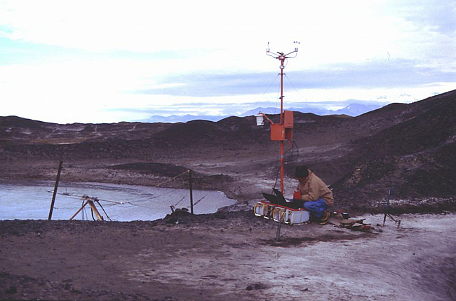
Ian Hawes downloading data from a climate station at Bratina Island.
Update 4: Environmental data. We are conducting a project to investigate relationships between Antarctic terrestrial species and their environment, and our ability to estimate these.
Our experimental approach involves constructing an ecological niche model for testing on eight Antarctic species grown in culture. The model seeks to explain the response of individual species to variations in environmental variables.
Building the model requires two types of input:
- distributional data for the eight chosen species in the Ross Sea sector (in this case the data come from the DNA sequencing of 250 samples from throughout this region, and they will be discussed in a subsequent update)
- environmental data for each of the sites (see the map below) from which the DNA sequences have been obtained.
The measurement or estimation of these environmental data is the subject of this update.

What to measure?
Many different environmental variables could be measured, but our project was constrained by several practical considerations. For a start, because our samples are ‘legacy’ material – collected by different individuals, at different times, for different reasons – the amount of data associated with them varies from considerable to almost zero. Data from the ‘almost zero’ samples therefore have to be collected by us, and to ensure consistency across all the samples we collected the same data from them all.
In addition, the kinds of data we can collect are restricted to those that can be measured from a sample that has been frozen and stored long term, and those that can be measured or estimated remotely using satellite technology. Finally, not all environmental variables are relevant to the distribution of species.
Given these practical constraints, we need to focus on the types of data that are likely to drive the distribution of species while satisfying the above criteria.
Salinity
Put simply, this is a measure of all the salts dissolved in water. We don’t just mean sodium chloride (table salt), but all the ions present. The cations (positively charged ions) in surface waters are typically dominated by sodium, followed by calcium and magnesium. You might not expect the non-marine habitats in the Ross Sea Sector to be very salty, but these ecosystems actually range from freshwater to more saline than seawater. Don Juan Pond, in the Wright Valley, is over 40% saline and is regarded as the saltiest water body on Earth. This pond is a saturated solution of calcium chloride, with sodium present in lower quantities. Life has been reported here, but it is very sparse.
Although Don Juan Pond is not one of our collecting sites, some of our samples came from very saline environments. In order to design laboratory experiments that accurately simulate these sites, we need to estimate (a) total salinity and (b) the proportion of ions that are monovalent, such as sodium (Na+), and the proportion that are divalent, such as calcium (Ca2+). (Monovalent and divalent ions can have different biological effects, and, as the example of Don Juan Pond shows, the proportion of each can differ.)
Fortunately, a useful proxy for total salinity is the electrical conductivity of the sample, and this can be measured simply using an inexpensive meter. To address (b) we made use of a chemical technique that measures the concentration of calcium and magnesium together. This is called titration, and works according to the diagram below. works to determine the concentration of divalent ions. For full explanation, see text.")
In brief, a blue dye is added to the sample, which turns pink in the presence of calcium or magnesium. The compound EDTA, which has a stronger affinity for these ions, is then added. EDTA scavenges the ions from the dye complex. When all the ions have been removed, the dye turns blue again. The amount of EDTA added to reach this point is proportional to the concentration of magnesium and calcium, which means we can calculate the proportion of divalent ions. A 30-second video showing the colour change can be viewed below.
Measurements using a conductivity meter and titration can be undertaken on samples that have been stored frozen, making them ideal to use on our legacy samples.
So, what did these measurements show?
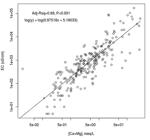
In the graph above, EC stands for ‘electrical conductivity’ and [Ca+Mg] means ‘the concentration of the two elements calcium and magnesium’. The important result is that the points fall near a straight line; this means that experimental salinity treatments can use a constant ratio of calcium and magnesium to sodium.
Bird life
Although microorganisms are widely distributed across Antarctica, prolific growths of flora (in quantities that can be seen with the naked eye) tend to occur in hotspots, such as where water is present, where conditions are warmer, or where nutrients are supplemented by bird life. Sites influenced by birds are coastal (e.g. Cape Hallett, shown below), and anyone who has visited a penguin colony is likely to remember the smell of ammonia, an inorganic nitrogen-containing compound. Bird guano is also a major source of phosphorous. Nitrogen and phosphorous are the two elements that most often limit the growth of plants – both terrestrial and aquatic.

However, measuring these nutrients in old samples is difficult. Ammonia, in particular, which is a good indicator of the presence of penguins, can disappear over time. At the other extreme, the indophenol blue method used for its measurement is inhibited when the ammonia is too concentrated – something that can happen when there is a lot of penguin-related contamination. The reaction can also be inhibited by other substances. Our attempt to use ammonia in the samples as a surrogate for penguins proved unreliable.
Luckily, DNA (which would be sequenced from the samples anyway) provides several alternative ways to estimate the influence of birds. One way is to look for DNA sequences of bird species in the samples; another is to look for DNA sequences of parasites, such as the invertebrate Stegophorus macronectes, whichinfects a range of Antarctic seabirds. Efforts to do this are proceeding: watch this space!
Liquid water
This is required by all known life, but a challenge for our project is how to estimate its availability from old samples that have been stored frozen. The work of Byron Adams (see the first update) and his colleagues has shown convincingly that the distribution of different nematode species is affected by water availability. For instance, Plectus murrayi is most often found in moist habitats, whereas Scottnema lindsayae is common in dry soils. Therefore, the ratio of DNA sequences from these two species in a sample will provide a measure of water availability. You might think that the water content of the sample could be used as a measure of its availability when it was collected, but storage conditions of a frozen soil can influence this variable over time.
Temperature
Temperature is of major importance in controlling the distribution of species. Temperature decreases overall with both altitude and latitude: with every 500 km of latitude south the mean annual temperature decreases by about 2°C. The effect of temperature on biota is easy to discern. Consider a local example such as the tree line, or trends observed in animals, such as those described by Allen’s Rule (roughly, animals adapted to colder climates tend to have shorter limbs) and Bergmann’s Rule (within a group of related animals, colder temperatures favour larger species).
However, the effect of temperature in Antarctica can be difficult to interpret. The trend of decreasing temperature further south is well established, but the international Latitudinal Gradient Project found that local effects tend to be more important than latitude in determining the distribution of biota. For instance, local variations in water availability can override the importance of temperature.
Temperature cannot be measured from our stored frozen samples, but it can be measured remotely thanks to satellite technology employed by Fraser Morgan’s team (see the first update for more information about Fraser). The data obtained in this way can be checked and calibrated using a network of climate stations present in Antarctica, such as those in the images below.
.")
Comments