Update 6: Testing predicted responses of Antarctic plants and microbes to environmental change
CAN WE PREDICT THE TOLERANCES OF ANTARCTIC SPECIES FROM THEIR FIELD DISTRIBUTIONS?
In Update 1 we explained our goal of experimentally testing the tolerances of Antarctic biota, as predicted from field distributions. Later you met the eight organisms being used in the tests. We showed you the collection of environmental data describing the habitats of these species, from which (by using their distribution patterns) we inferred their tolerances. The last update illustrated the growth of organisms in culture, and showed how growth rates can be measured on agar plates and compared across treatments (such as different salinities, or the presence or absence of simulated penguin excreta).
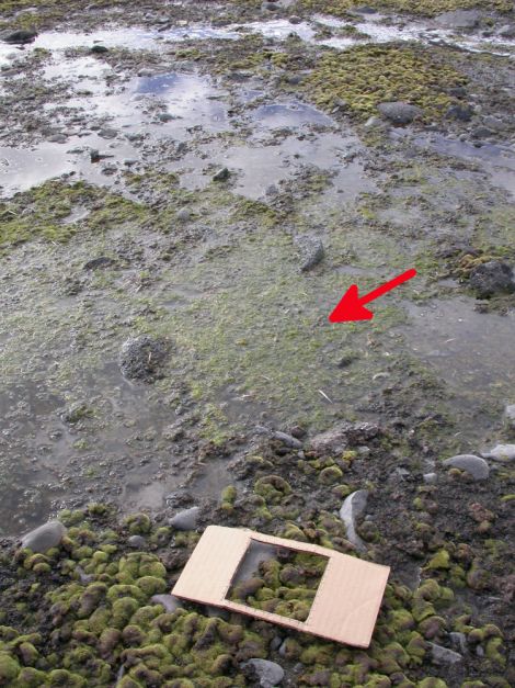
Now it’s crunch time. Let’s compare the tolerances we inferred from field distributions with what we observe in culture. To illustrate the point, we’ll consider a simple example: Prasiola. This is a green alga, well known from penguin rookeries, where it can grow in great abundance (much greater than is seen elsewhere). From this we would infer that penguin excreta has a large positive effect.
So what did we find when we cultured Prasiola?
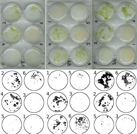
Even using the naked eye it seems clear that this species of alga responds positively to simulated penguin excreta. However, we can quantify this effect using pixel counts:
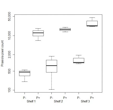
Although the effect of penguin supplementation is very dominant (and more so than it appears, since the vertical scale is logged, making larger numbers seem more similar), the plot above enables us to see that growth also increases slightly as one progresses up the shelves. This could be caused by a temperature gradient in the incubator, or slightly different positioning of the plates with respect to the lights. Accounting for such unforeseen “errors” is why we use replicate treatments – otherwise the errors would be invisible – and also why we randomise the treatments within each shelf.
Above we have considered a single day, when in fact the experiment ran for 45 days with repeated scans of the plates. We can produce growth curves for this experiment over time:
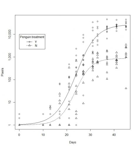
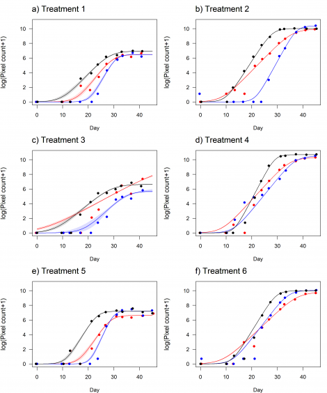
The growth curves shown above have three parameters: the lag (the distance after the start at which the curve starts to go up), the maximum growth rate (the slope of the line at its steepest point), and the asymptote (the pixel value at which the line levels off).
The effect of the simulated penguin treatment is easy to see in this example, because it is so dominant. However, it is not the only treatment in the experiment: we also have salinity, and ultimately temperature (which requires experiments that are still going on to be completed).
To show the effects of all the treatments we have to compile quite a complicated model. Basically, the three parameters mentioned above are modelled as combinations of the treatments. Let’s look at the output of one of these models:
So, for instance, we can describe the effect of the treatments (increasing salinity, the simulated presence of penguins, and the interaction between these two things) on the maximum biomass. The ‘penguin present’ effect is interpreted as the change in maximum biomass relative to the treatment with no penguins. The ‘salinity’ effect describes the steepness of a line that relates salinity to the maximum biomass when there is no penguin treatment. The interaction describes how the slope of that salinity line varies when there is a simulated presence of penguins.
The model also allows for the effect of replicates being on different shelves. This step is important, because if growth was very different between shelves, not accounting for it would mean that the data would be too noisy to detect any potential effects of the treatments that interest us (i.e. salinity and the simulated presence of penguins. However, that’s not the case here. The confidence intervals allow us to state that the effects of various treatments are statistically significant. So let’s summarise the significant parameters.
The effect of adding simulated penguin excreta on the maximum biomass attained is significant.
The interaction effect of adding simulated penguin excreta on higher salinity is also significant. This is like saying, if salinity is higher, the effect of penguin presence is to shorten the lag phase. In other words, the population starts going up sooner.
Finally, the effect of raising the salinity on the growth rate is significant. However, the results show that salinity is much less important than adding simulated penguin excreta in these experiments – and, presumably, in the field as well.
Look out for one more update in the next month or two, when we incorporate temperature into the model. This could be the most important effect, and the most directly relevant in the context of climate change. So stay tuned!
